The duality – Geometric Algebra

The concept of duality in physics is extremely interesting because it connects aspects that can be considered opposites , by means of a correspondence which instead it leads to identify oneself in the formal aspect, or in the equations.
In this sense, duality is the best translation of the suggestive concept of coincidentia oppositorum of the medieval philosophical tradition.

In physics, duality is largely found in electrical phenomena:

voltage – current
circuit series – circuit parallel
resistance $R$ – conductance $G$
voltage divider – current divider
impedance $Z$ – admittance $Y$
capacity $C$ – inductance $L$
reactance $X$ – susceptance $B$
short circuit – open circuit
Kirchhoff’s current law at a node – Kirchhoff’s voltage law in a loop
Thévenin’s theorem – Norton’s theorem

In addition to a speculative interest, the principle of duality has a practical implication much loved by students because it allows you to memorize only half of the formulas, because the dual ones are immediately obtainable. For example the capacitor is characterized by this constitutive relationship:

$\begin{equation} i_C = C \frac{d}{dt} V_C$

knowing that inductance is the dual quantity of capacitance and that voltage and current are also dual quantities, the dual relation is immediately obtained:

$\begin{equation} V_L = L \frac{d}{dt} i_L$

Finally the principle of duality is a heuristic principle, that is, it serves to discover something new.
In 1825 the French mathematician Joseph Gergonne noticed that for every theorem in projective geometry that involved lines and points, a dual one corresponded, that is, obtained by exchanging the roles of lines and points. For example to the theorem “two points define a line” corresponds “two lines meet at a point” or “three points define a plane” corresponds “three planes intersect at a point”.

In algebra the notion of duality corresponds to the orthogonal complement , i.e. the subspace formed by all the bases that do not constitute the element.

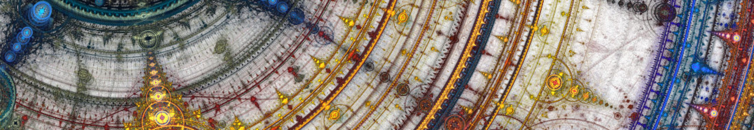
The duality relationship is so important in GA that it has a dedicated symbol $^*$ (star). The dual of a multivector is obtained by multiplying to the right by the inverse of the unitary pseudoscalar $M^* = M I^{-1}$ (definition used by Hestenes and which we find in the texts of A. MacDonald – see references).
Other authors, for example Doran in [7], use the definition $M^* = M I$ which is equivalent.

For example, the dual of the plane identified by the bases
$(e_1 e_2)^* = - (e_1 e_2)(e_1 e_2 e_3) = e_3$
If instead we start from the vector $e_3$ we will have to use the inverse transformation $M = M^* I$ and therefore
$(e_3)(e_1 e_2 e_3) = e_1e_2$
therefore it is necessary to pay attention to the direction in which we are carrying out the duality operation: from vectors to bivectors or the other way around.

Transformations of duality in 3D geometric algebra

It is interesting to note that where $I^2 = -1$ , therefore in 2D and 3D, the dual of the dual of an element does not coincide with the element itself: there is a minus sign to make the difference. For example
$(e_2)^* = - I e_2 = - e_1e_2e_3\: e_2 = e_1e_3$
$(e_2)^{**} = (e_1e_3)^* = - I e_1e_3 = - e_1e_2e_3\: e_1e_3 = -e_2$
therefore it takes two cycles of duality to bring us back to the original element.
In general in a n-dimension space $n$ we will have $M^{**} = (-1)^{n(n-1)/2} M$ .

Duality relationships between vector and bivector bases in 3D (the signs reflect the definition of the dual $M^* = MI$ )

Duality relationships between vector and bivector bases in 3D (the signs reflect the definition of the dual $M^* = MI$ )

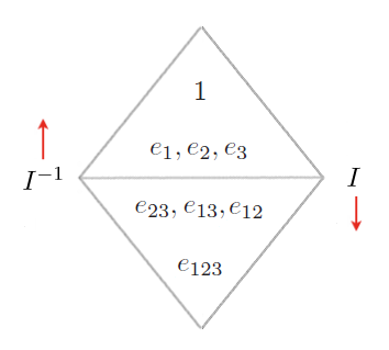
The duality relation has been used unconsciously for decades in vector algebra: in fact the phantom axial vectors are nothing more than masked bivectors, as can be seen in the figure

As an exercise, we calculate the dual of the external product $\pmb{a} \wedge \pmb{b}$ :

$(\pmb{a} \wedge \pmb{b})^* = (\pmb{a} \wedge \pmb{b})\: I^{-1} = - (\pmb{a} \wedge \pmb{b}) \: I = - I (\pmb{a} \wedge \pmb{b})$

since in 3D the pseudoscalar I switches with each element. Therefore, by carrying out:

$(\pmb{a} \wedge \pmb{b})^* = - e_1e_2e_3 \: [(a_1 b_2 - a_2 b_1) e_1e_2 + (a_1 b_3 - a_3 b_1) e_1e_3 + (a_2 b_3 - a_3 b_2) e_2e_3]$
$= - (a_1 b_2 - a_2 b_1) e_3 + (a_1 b_3 - a_3 b_1) e_2 - (a_2 b_3 - a_3 b_2) e_1 =$
$= [(a_2 b_3 - a_3 b_2) e_1 - (a_1 b_3 - a_3 b_1) e_2 + (a_1 b_2 - a_2 b_1) e_3] = (\pmb{a} \times \pmb{b})$

We recognize the classic vector product in the final expression!
Therefore between the external product and the vector product there is a relationship of duality.
The inverse relationship also holds: $(\pmb{a} \times \pmb{b})^* = - (\pmb{a} \wedge \pmb{b})$

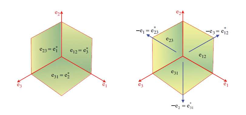
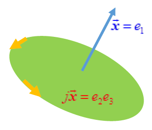
It is important to underline a difference between the dual of a multivector and its orthogonal complement. The dual maintains a relationship of extension and orientation with the multivector, for example between the plane and the vector perpendicular to it, which will have a modulus proportional to the area of the plane and a coherent orientation. The orthogonal complement, on the other hand, being a subspace, extends to infinity and is not oriented.