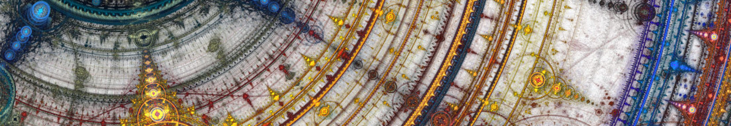
Let us now deal with the motion of the planets, which responds to the universal law of gravitation discovered by the great Isaac Newton. We schematize the situation with two bodies of mass  and
and  which are at a certain distance
  and
and  with respect to a point taken as a reference.
The reciprocal distance  is worth
  (vectors, of course). These two bodies attract each other with a force directed along the connecting line, whose intensity varies with the inverse of the square of the distance and is proportional to their masses:

To put it simply, will be much larger than , as is the case with planets around the Sun or satellites around their planet. So we can write the alternative, more compact form for the acceleration of :

Where  and the sign is justified by the fact that the vector radius goes from to .
If we start with the body stationary, the motion would simply be a fall of accelerated motion and would take place along the segment containing the two centers. Nothing interesting, then.
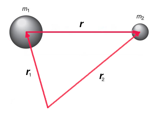
This becomes interesting when the body has an initial velocity in a direction other than that of . If this happens, the body is endowed with a quantity which is called angular momentum.
In the classical treatment this quantity arises from the vector product between the vector radius and the momentum  :
:

and the result is an axial vector, which – we have already said – is not our cup of tea.
So we prefer to express it in a more appropriate way to geometric algebra as the external product between and and therefore it is a bivector:

As a bivector, it geometrically expresses the area swept by the vector ray during the motion of the body around  .
.
A naturalist studies Nature by observing the strange animals he encounters and examines them to see their behavior: how they move, what they eat, what sounds they make, how they reproduce. Physicists work in exactly the same way. First of all, let’s see how L changes over time: to know it, let’s calculate the derivative, which as a linear operator, acts on the external product just like in the case of the product of two terms:

The last step is justified by the fact that the gravitational acceleration is directed exactly in the direction and therefore the external product is zero. In conclusion: in gravitational motion the angular momentum is conserved. First important consequence: the motion takes place in an invariable plane.
From this first consideration, if we take into account the geometric meaning of the angular product, we can already justify Kepler’s second law, namely that the area swept by the vector ray is a constant quantity over time.
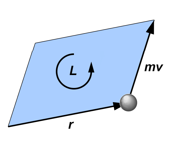
Now let our planet move with speed  in a generic direction: we see that in the infinitesimal time
  the vector radius describes an area equal to that of the triangle, that is half of the parallelogram with sides ed
  or
or

or also, rearranging:

therefore the areal velocity is equal to half of the angular momentum.
Another constant of motion
Now we want to develop that external product  which defines the angular momentum.
Our main tool will be the technique of decomposing any vector  as the product between its module and the versor
  because by doing so, when we consider the generic variation of a vector quantity, we are able to separate the contribution due to the change in length and to the change in direction. To put it in courtly terms, let’s separate the contributions of intensity and geometry.
So:  and therefore:

but since is the derivative of  then using the derivative property of a product:

but in the development of the expression the first term is null because  and therefore remains:

at this point we recall the definition of the geometric product between those versors:  , then:

Now imagine we are observing the  unit vector: we must necessarily conclude that any variation, not being able to concern the module, will concern the direction and therefore the vector of its variation over time
  will necessarily be perpendicular to and hence their dot product
  is null. So:

We need this expression to derive another constant for planetary motion. To find it, let’s go back to the law of gravity:

and neatly multiply the two members with the found expression for the angular momentum, relieved to find that many terms cancel each other out ( ):
):

We can write it in the form  or, in the differential way:

So the quantity  , and has a vector nature because since
  is a bivector, and recalling what we said before, the vector will be rotated
  clockwise (and scaled) by the bivector on its left.
This constant vector is known as the Laplace-Runge-Lenz vector , denoted by  in the following figure. As can be seen, it is constant and directed towards the perihelion.
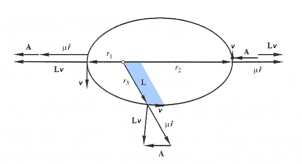
Planet’s trajectory
Let’s work out this interesting constant vector by multiplying it to the right by the vector :

Carrying out all the geometric products:

the last term lacks the wedge because and have the same direction.
Remembering that  :
:

From the point of view of degrees, this equation is composed of:
bivector + scalar = scalar + bivector + scalar
therefore we are going to equal the scalar terms (note:  is positive because the square of a bivector is negative!):

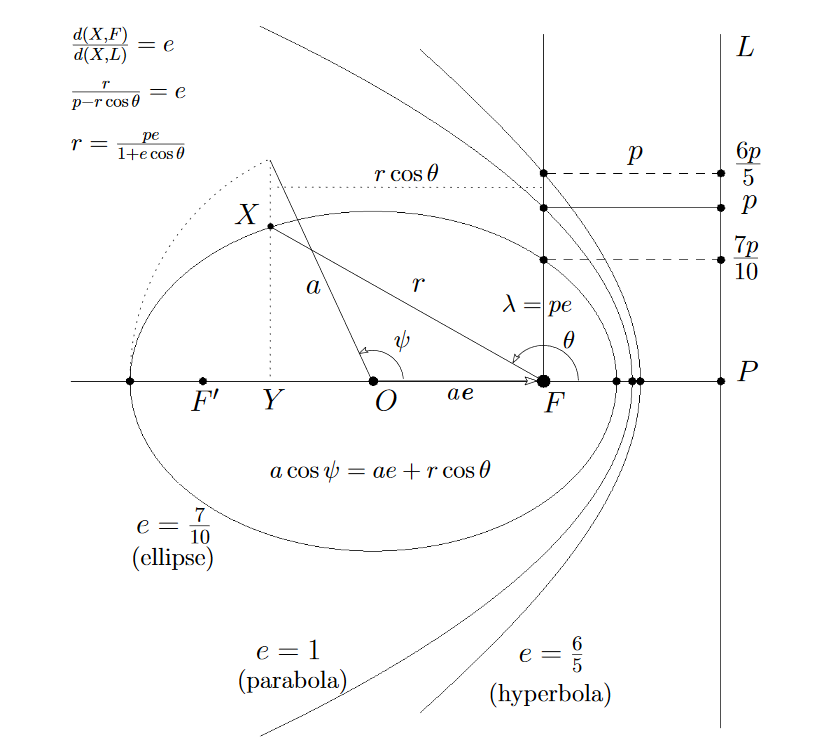
and we recognize the polar equation  :
:

very similar to the equation of a conic in polar form, to which we can easily lead back:

Let’s redefine  (semilatus rectum) and
  (eccentricity):


Here is the trajectory revealed, with its main parameters:
Now let’s think of the body in elliptical motion around which occupies one of the foci.
It will describe the dotted triangle at some time and this depends on the angular momentum L because we have seen that

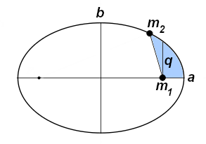
Over the entire orbital period  will describe the area
  , but then:

rearranging and switching to squares:

and from the geometric properties of the ellipse, we know that  and we also know that

and then:

By simplifying and rearranging, we finally get Kepler’s third law:
