In the 1990s, computers were often equipped with a program that made its users spend hours and hours of delight. Incredibly, we’re not talking about a video game, but Fractint. It was a free program that could calculate fractals incredibly fast and then with the +, – and <space> a psychedelic show started in which the extraordinary shapes were animated by breathtaking colors, creating very creative trips.
The extraordinary shapes of the Mandelbrot or Julia set are generated by a very simple iterative formula in the complex numbers domain: 
The fundamental question is: how can such rich forms derive from a very simple formula? The secret lies, of course, in the iteration, which also explains the repetition of motifs within the fractal’s structures, as if they were musical variations on a theme or the elaborations of a temple’s ornaments. It is worth clarifying that there are different mechanisms for generating fractals: iterated function systems (IFS), for example, repeat a set of contractive affine transformations and produce attractors such as the Barnsley fern or the Sierpinski triangle. The Julia and Mandelbrot sets, instead, arise from a different mechanism: the iteration of a single quadratic map  , which is not contractive at all — on the contrary, outside the set the sequence diverges, and it is precisely this that traces its boundary. It is on this latter mechanism that we focus.
Let’s focus on Julia’s set: for each point  of the complex plane, we compute
  and then add a fixed constant
  for all points. The number we get will be the starting point for another iteration. The behavior of this sequence is very variable: it can explode towards very large numbers, or remain contained, let’s say within a radius
  from the origin. If after a certain number of iterations the sequence does not diverge, we affirm that the point belongs to the fractal.
As a further refinement, we can assign a shade of color based on the value of the sequence at the end of the calculations.
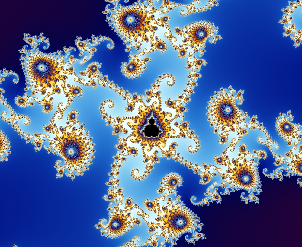
One of the possible results (which depend on the choice of ) is the following, obtained with  and a limit of 50 iterations:
After presenting the “classical method” fractals, we want to achieve a goal halfway between the absurd and the useless, but with the prospect of finally being able to understand the characteristics of fractals. We want to eliminate complex numbers from fractals, transforming them into vector operations and therefore potentially applicable in reality, for example on a sheet of paper.
As already said, if we want to correctly vectorize a complex number, we must multiply it by the base which for us identifies the direction of the real axis (say  ):
): 
Then the Julia fractal formula in vector form will become:

which is equivalent (multiplying to the right by  ) and considering that
  to the equation:

which expresses a geometric fact: the next vector of the iteration is equal to the reflection of the base with respect to the previous vector to which the constant vector is added.
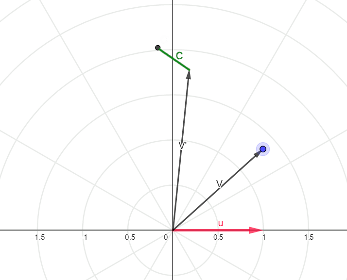
Then we can generate the Julia fractal in this way: for each point of the plane represented by the vector  we mirror the base on this vector, we scale it by a factor
  and then add . The resulting vector will be subjected to the same operations until the fixed iteration limit is reached.
If the result is bounded (say inside the circle of radius 2), then the starting point belongs to the Julia set.
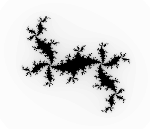
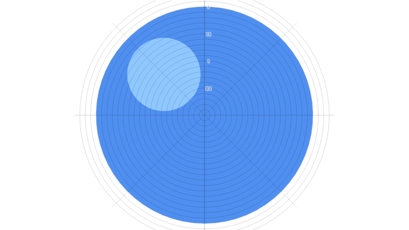
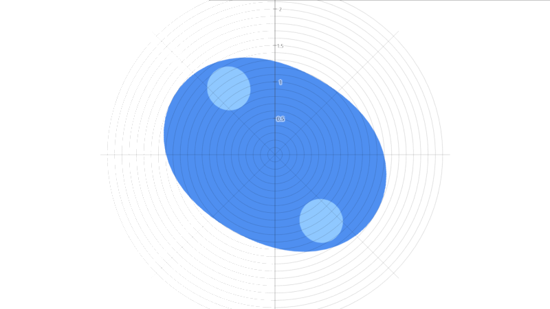
Let’s look at the overall result: some points of a shape that we do not know at the beginning of the process (in fact, only at the end of the iterations do we know if the point belongs to the set or not) are mapped into the circle of radius 2. So let’s do it smart: to generate the Julia set we start from the circle of radius 2 and reverse the process!
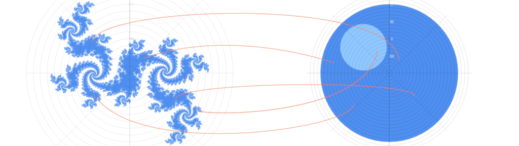


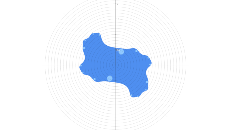
The new process will therefore be: we will start from the circle of radius 2, we translate it in the opposite direction with respect to and at this point we apply the inverse transformation: the new vector will be on the bisector between the old vector and and the module will be its square root.
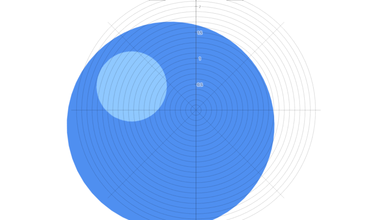
 shift
shift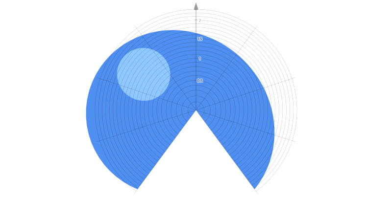
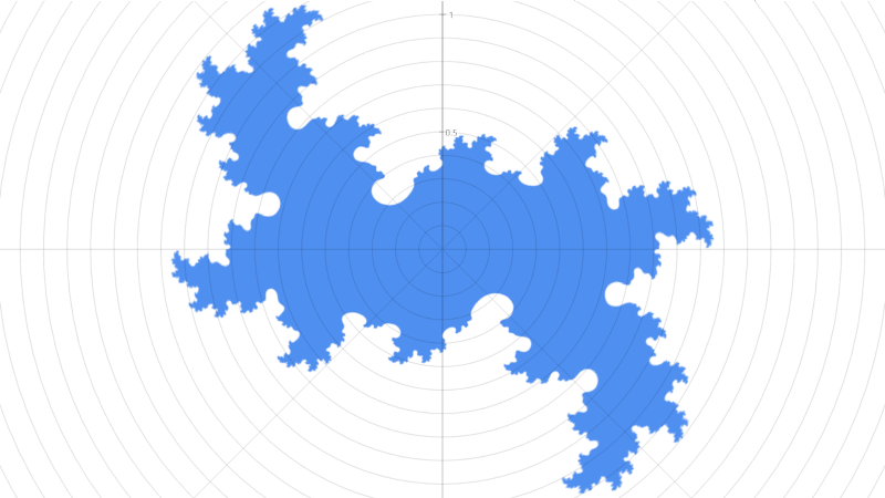
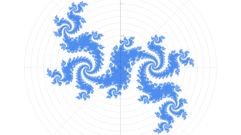
Sequence from Steven Wittens’ excellent post “How to fold a Julia fractal“.
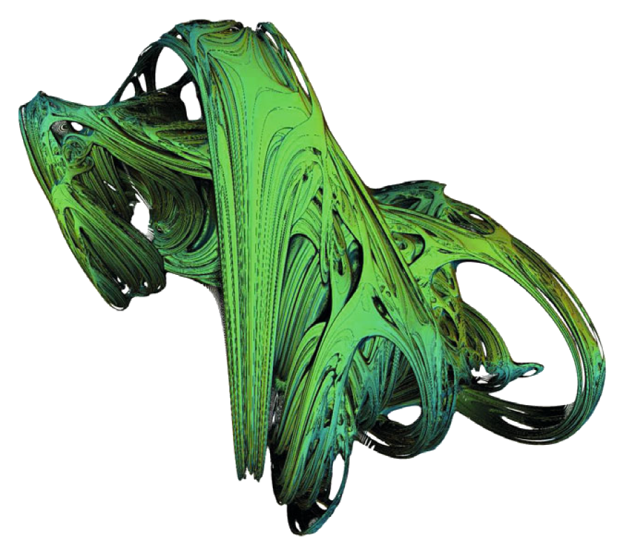
The extraordinary fact is not only that we have produced a fractal without resorting to complex numbers, but also the fact that – as already said – the GA scales dimensions without difficulty and in fact we can apply the same formula in 3D and we obtain a Julia fractal 3D, without further effort.
If the result is nice, well … is a different kettle of fish.
Generating Fractals Using Geometric
Algebra 2011