Spacetime and relativity – Geometric Algebra

In 1907, the German mathematician Herrmann Minkowski became convinced that the newborn theory of relativity of his former pupil Einstein, based on previous works by Poincaré and Lorentz, could be represented in a four-dimensional space-time but not Euclidean, because time had to be distinguished from spatial dimensions.
The following year he fully formulated his theory and summarized it in the famous phrase “henceforth space by itself, and time by itself, are doomed to fade away into mere shadows, and only a kind of union of the two will preserve an independent reality“. This new representation proved extremely useful and helped Einstein a lot in the next step, that is, extending relativity to gravitation.

In geometric algebra, therefore, we will exploit for the first time that footnote hidden in one of the axioms: the product of two bases must be a real number. We did not say positive, in fact the base that identifies with time will be distinguished from space precisely by the sign of the square.
We will then have four bases, which change letter because this is the notation established in relativity:

$(\gamma_0, \gamma_1, \gamma_2, \gamma_3) \mapsto$ (time, 3 spatial coordinates)

The first tool we need is the vector norm, which is how much $a \cdot a$ is worth. The sequence of the four signs of each component is called signature and in theory we would be free to choose the one preferred by relativistic physicists (-, +, +, +) or the one preferred by particle physicists (+, -, -, -). No physical theory would allow the two to be distinguished: they produce the exact same results.
In the case of the GA, however, this freedom does not exist: if we want the algebra to be consistent, we must choose the latter, because it is the only one that manages to correctly include the subalgebra of three-dimensional space! Therefore:

$|a|^2 = a \cdot a = \gamma_0^2 - \gamma_1^2 - \gamma_1^2 - \gamma_3^2$

This mixed signature opens up some novelties: a vector can have null “length” (vector of light type) or even negative (vector of space type). In some texts it is stated that this is all that is needed to formulate a physical theory in the relativistic field, but then technical difficulties are encountered when it is necessary to model the electromagnetic field and the angular momentum. We end up having to resort to more complex mathematical tools (antisymmetric rank 2 tensors). But we know well that geometric algebra has an additional arrow to its arc: the geometric product. It is precisely this – we will see – that simplifies the work extraordinarily, avoiding the use of tensors.
It’s an investment that pays off big time!

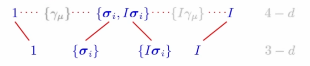
Then the other components of the algebra of spacetime (abbreviated to STA) will be born.

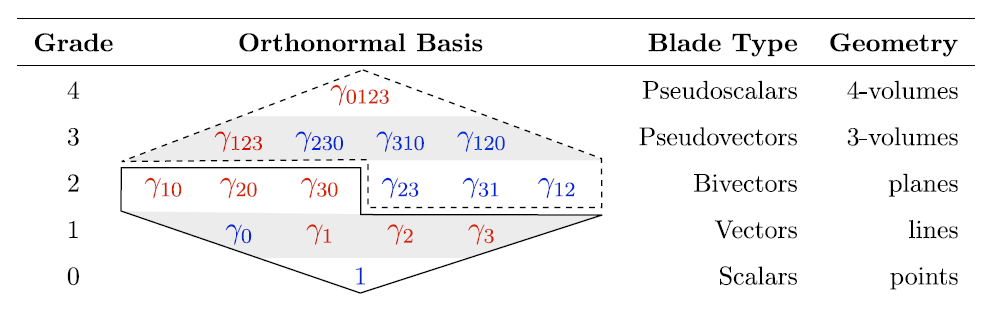
The color of the elements indicates the signature: positive in blue, negative in red.
The areas enclosed by the solid and dashed lines are mirrored in the duality relationship (multiplication on the right by the pseudoscalar $I = \gamma_{0123 }$ ) while inside the same box, the light and gray background areas are mirrored in the temporal duality (multiplication on the right by the base $\gamma_0$ ).
Note that the temporal bivectors are indicated as $\gamma_k \gamma_0$ : the reason will be clear in the following.

It is remarkable that even in the STA the pseudoscalar $\gamma_{0123} ^ 2 = -1$ and therefore we can indicate it once again with the symbol $I$ . Furthermore, $I = I^*$ and anticommutes with vectors and trivectors while, as always, it commutes with all elements of even degree.
The generic multivector will therefore be the combination of all degrees:

$M = a + v + B + T + \beta I$

but we will exploit the duality to reduce it to the complex form:

$M = \zeta + z + B = (a + \beta I) + (v + wI) + B = (a + \beta I) + (v - wI) + B$
con la particolarità che $T = wI = -wI$

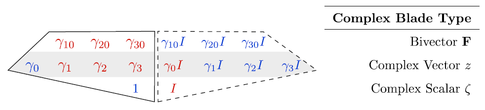
The complex structure halves the degrees of the STA leaving the bivectors as irreducible entities, which cannot be further broken down.

Bivectors in STA

Therefore the undisputed protagonists of the STA are the bivectors.
The three basic bivectors of space type, as we have already seen, have a negative square and the fundamental identity holds:

$e^{\theta \gamma_j \gamma_k} = \cos \theta + \sin \theta \: \gamma_j \gamma_k$

sequence of rotations generated by a purely spatial bivector

and then generate ordinary rotations.

On the other hand, the fact that there is a time base $\gamma_0$ between the components of the three space-time mixed bivectors determines a substantial difference: this time the square of the bivector is positive. Positive norm bivectors have a number of new properties, compared to those we already knew and the most important is this:

$e^{\theta \gamma_k \gamma_0} = \cosh \theta + \sinh{\theta} \: \gamma_k \gamma_0$

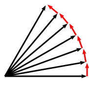
therefore in these bivectors we are dealing with a hyperbolic geometry, in fact they do not generate a rotation and we see it well with two simple tests:

$\gamma_1 (\gamma_1 \gamma_0) = -\gamma0$
$\gamma_0 (\gamma_1 \gamma_0) = -\gamma1$

the pseudo-rotation generated by the mixed bivectors is called with the English term boost which means speed variation.

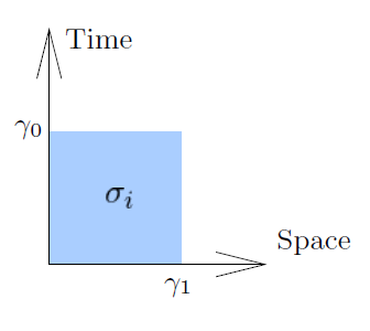
boost sequence generated by a space-time bivector

It should be noted that to respect the tradition that sees these diagrams with time on the ordinate and space on the abscissa, the bivector should be indicated as $\gamma_k \gamma_0$ or right-handed.
These spacetime bivectors have a dedicated notation:
$\sigma_i = \gamma_i \gamma_0$
their importance derives from the fact that – even if they are properly bivectors – they are to be considered vectors in the reference system perpendicular to the time axis $\gamma_0$ and for this reason they are called relative vectors, where the relative adjective is to be understood as with respect to the speed of the reference system.
Therefore, given a space-time bivector, it will be sufficient to multiply it to the right by $\gamma_0$ to extract the spatial component $\gamma_i$ in that reference system.
More generally, $\gamma_0$ determines the mapping of each spacetime vector $a = a ^ \mu \gamma_\mu$ as:

$a \gamma_0 = a \cdot \gamma_0 + a \wedge \gamma_0$

therefore the scalar is the time component of the vector a and the bivector can be decomposed into the bases $\sigma_k$ and represents a space vector relative to the observer of the reference $\gamma_0$ .

The letter $\sigma$ is not taken at random, because these spacetime bivectors behave exactly like the Pauli matrices, developed to explain the phenomenon of spin in quantum physics.

As we have seen in the 2D and 3D cases, the even subalgebras have an importance deriving from the fact that they are isomorphic to known algebras, respectively to $\mathbb{C}$ and to $\mathbb{H}$ , that is to complex numbers and quaternions.
The even subalgebra of the STA is made up of scalars, 6 bivectors and the pseudoscalar.
It is interesting to note that these elements can be mapped in the ordinary algebra of three-dimensional space! In fact, the pseudoscalar is the same: $\sigma_1 \sigma_2 \sigma_3 = (\gamma_1 \gamma_0) (\gamma_2 \gamma_0) (\gamma_3 \gamma_0) = \gamma_0 \gamma_1 \gamma_2 \gamma_3$

The relative vectors map to the ordinary 3D vectors and the relative bivectors to the ordinary 3D ones.
This interesting decomposition is observer-dependent, because everything is linked to the specific time axis $\gamma_0$ .