Geometric resolution of 2nd degree equations

In the first two grades of high school, second degree equations and the formula for their solution are presented, while limiting the treatment to real solutions.
Here we want to present a general method of geometric resolution of all second degree equations, even those with $\Delta <0$ using an app made in geogebra. The aim is to show how usefully the two worlds of translation and rotation are complementary.

Click to open the Geogebra app

Let’s start from the classic second degree equation $x^2-1 = 0$ which admits two real solutions $x_ {1,2} = \pm 1$
Students are trained to transform these equations into parables and to recognize the intersections with the axes, the symmetries, the position of the vertex in analytic form. In this way, starting from algebraic geometry, they build those mathematical capabilities essential for scientific studies.
We could say – with a play on words – that geometric algebra complements this training by geometrizing mathematics.

For this exercise, in fact, we want to see that equation in a much more naive form. In very simple terms, it says, “let’s take an unknown quantity $x$ , square it and subtract one unit. If all of this comes out zero, then that $x$ quantity is exactly what we’re looking for.” We can imagine that this story takes place along the real axis: then we will have two quantities that add algebraically (we can use two vectors) and we will be satisfied when the sum coincides with the origin.

After setting up the app (check the “Re” box to indicate the real solutions and the correct coefficients) you can act on the slider that tests all the values of $x$ : you can verify that the $V$ value of the function will coincide with the origin when $x = \pm 1$ You can play freely, for example with the equation $x^2 - 3x + 2 = 0$ to find the solutions geometrically.

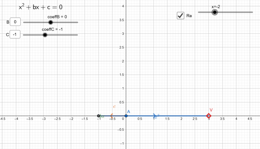
If we now represent the equation $x^2 + 1 = 0$ we realize that the point V never manages to reach the origin. We must access a further degree of freedom: that is, to be able to rotate the vectors in the plane, as well as scale them: this is the only way to reach the origin.
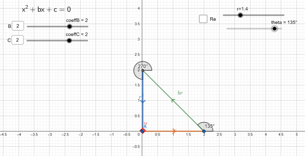
If we uncheck the “Re” checkbox, an extra slider will appear, which corresponds to the second parameter of our unknown: the angle of rotation. So now we will not denote the unknown with the $x$ expressing only a real number with a sign, but we will indicate $r \angle \theta$ or even better $r e^{i \theta}$

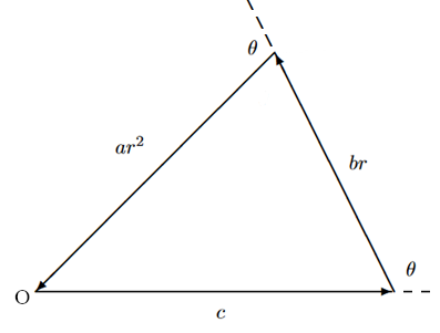
It remains to understand how to represent the terms of the equation when the unknown is a rotation: if the known term is a simple real vector and the linear term is a vector scaled by $r$ and rotated by $\theta$ , the quadratic term will be scaled by a factor of $r^2$ and rotated by $2 \theta$ (angles sum up).
These three vectors add up and if the figure closes in a triangle, that is, in the origin, the rotation $r \angle \theta$ is a solution of the second degree equation.

Let’s try the equation $x^2 - 2x + 2 = 0$
The triangle closes when $r \approx 1.4$ and $\theta = 135^\circ$ or $\theta = -135^\circ$ because the two solutions are symmetric, if the coefficients of the equations are real (cf. fundamental theorem of algebra).

Of course this is only a visual demonstration: in secondary school you have all the tools to be able to proceed to a geometric-analytical resolution. In fact it is clear that the triangle is necessarily isosceles and therefore we immediately obtain $r = \sqrt {c / a}$ furthermore the perpendicular to the linear vector divides it into two halves and therefore with the Pythagorean theorem we also find the angle $\theta$ .

For example for the case illustrated above, $r = \sqrt{2}$ and it turns out that the equal angles are each worth $\pi / 4$ and therefore the solutions are $\sqrt{2} \angle \pm 3 \pi / 4$
If you really want the complex number, you can easily find that $x_ {1,2} = -1 \pm i$ but at this point it will be evident that we consider complex numbers as rotations + dilations manages to enrich a purely algebraic problem with a geometric sense.