Maxwell’s equations – Geometric Algebra

Maxwell’s equations had a very complex history, mainly because as the theory of electromagnetism developed, so too did the mathematical techniques used to describe it.

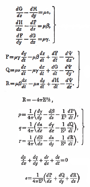
In the first publication of 1861-62, still steeped in mechanical analogies, Maxwell published these 12 equations. Later they rose to 20, but these also included phenomena (for example Ohm’s law) that we now exclude from Maxwell’s “fab four” equations.

Then, since they were the fashion of the moment, Maxwell tried to rewrite them in the form of quaternions, but was criticized by his enthusiastic supporter Heaviside, who instead proposed, together with Gibbs, a version in pure vector form, reworked from the quaternions, but very much more effective:

no sum of scalars and vectors (as the quaternions were conceived by Hamilton)
positive quadratic form
multiplication between vectors in the form of a scalar and vector product
notation still in use today

$\begin{equation} \nabla \cdot \vec{E}} = \frac{\rho}{\epsilon_0}$
$\nabla \cdot \vec{B} = 0$
$\begin{equation} \nabla \times \vec{E} = - \frac{\partial \vec{B}}{\partial t}$
$\begin{equation} \nabla \times \vec{B} = \mu_0 \left ( J + \epsilon_0 \frac{\partial \vec{E}}{\partial t} \right )$

The revolution of the theory of relativity, however, triggered by the same Maxwell equations that appeared in a covariant form, that is compatible with the postulates of relativity, led to their reformulation in the form of a tensor.

And now we come to the form of Maxwell’s equations in the key of GA. The tensors have been replaced by bivectors and the complex numbers are incorporated into the structure of GA itself.
Let’s start with the ingredients: the sources of the electric field are the charges and the (densities of) currents, condensed in the multivector

$J = \rho - \pmb{J}$

from the dimensional point of view, however, the right hand equation has a problem: $[C] [m] ^ {- 3}$ vs $[C] [s] ^ {- 1} [m] ^ {- 2}$ and we remedy the following:

$J = c \rho - \pmb{J}$

Then the absolute protagonist of electromagnetism: the electromagnetic field, as known in GA is worth $F = E + iB$ but even here we would have dimensional problems $[F] [C] ^ {- 1}$ vs $[F ] [C] ^ {- 1} [v] ^ {- 1}$ so we change it to:

$F = E + icB$

This is a very little traumatic modification: some authors, including Gauss, have proposed to indicate the magnetic field with the expression $cB$

Drum roll: Maxwell’s four equations become one:

$\begin{equation} \nabla F = \frac{1}{\epsilon_0 c}J$

With the clarification that the $\nabla$ operator must be understood here in a space-time sense, that is:

$\begin{equation} \nabla = \frac {1} {c} \frac {\partial} {\partial t} + \frac {\partial} {\partial x} \hat {x} + \frac {\partial} {\partial y} \hat {y} + \frac {\partial} {\partial z} \hat {z}$

This equation not only has the advantage of compactness, it has above all the relativistic invariance that comes from multiplying the quantities $\rho$ and $B$ by $c$ .

We now show how Maxwell’s four ordinary equations can be derived.
Expanding the definition of the ingredients seen above:

$\begin{equation} \left (\frac {1} {c} \frac {\partial} {\partial t} + \nabla \right) (E + icB) = \frac {c \rho - J} {\epsilon_0 c}$

as a second step, we distribute the product on the left:

$\begin{equation} \left( \frac{1}{c}\frac{\partial E}{\partial t} + \nabla E + i \frac{\partial B}{\partial t} + ic \nabla B \right ) = \frac{c \rho - J}{\epsilon_0 c}$

The two terms $\nabla E$ and $\nabla B$ expand by remembering the geometric product:
$\nabla \pmb{a} = \nabla \cdot \pmb{a} + \nabla \wedge \pmb{a}$

$\begin{equation} \frac {1} {c} \frac {\partial E} {\partial t} + \nabla \cdot E + \nabla \wedge E + i \frac {\partial B} {\partial t} + ic \: \nabla \cdot B + ic \: \nabla \wedge B = \frac {c \rho - J} {\epsilon_0 c}$

This monstrous equation can be rearranged as follows, with the purpose of ordering the terms by degree:

[NB: $ic \: \nabla \cdot B$ has the nature of a trivector because it is multiplied by the pseudoscalar i, while $ic \: \nabla \wedge B$ has the nature of a vector for the same reason!]

$\begin{equation} \underbrace{\nabla \cdot E}_\text{scalar} + \underbrace{\frac{1}{c}\frac{\partial E}{\partial t} + ic\: \nabla \wedge B}_\text{vector} + \underbrace{ \nabla \wedge E + i \frac{\partial B}{\partial t}}_\text{bivector} + \underbrace{ic\: \nabla \cdot B}_\text{trivector} = \frac{\rho}{\epsilon_0} - \frac{J}{\epsilon_0 c}$

now we just need a very simple observation:
scalar + vector + bivector + trivector = scalar + bivector
therefore we can express the relative equalities for each degree

$\begin{equation} \nabla \cdot E = \frac{\rho}{\epsilon_0}$

$\begin{equation} \frac{1}{c}\frac{\partial E}{\partial t} + ic \nabla \wedge B = -\frac{J}{\epsilon_0 c}$

$\begin{equation} \nabla \wedge E + i \frac{\partial B}{\partial t} = 0$

$\begin{equation} ic \nabla \cdot B = 0$

The first equation, as it stands, expresses Gauss’s law.

There is a bit of work to do for the second equation: first divide it by $c$ , knowing that $c ^ 2 = \frac {1} {\epsilon_0 \mu_0}$ and calling up the dot product $a \times b = i (a \wedge b)$ we will get the form:

$\begin{equation} \epsilon_0 \mu_0 \frac {\partial E} {\partial t} - \nabla \times B = - \mu_0 J$

at this point we isolate the rotor of B and obtain Ampère’s law:

$\begin{equation} \nabla \times B = \mu_0 \left (J + \epsilon_0 \frac {\partial E} {\partial t} \right)$

Also in the third equation we transform the external product into the vector one and we separate E and B, obtaining Faraday’s law:

$\begin{equation} \nabla \times E = - \frac {\partial B} {\partial t}$

and the last equation will simply be:

$\nabla \cdot B = 0$

… and tell me this isn’t wonderful !

Not only that: what we have seen could seem an exercise in style, as beautiful as it is useless.
It seems that to do the calculations you have to go back to the dear old equations: in reality the geometric product has sufficient power to express calculations and the ethereal equation $\nabla F = J$ can be solved with Green’s functions, more easily!

For example, if we are solving an electrostatics problem in two dimensions, therefore without charges within the region considered, we will have $\nabla F = J$ and by means of Green’s functions we will have to solve:

$\begin{equation} F (x) = \frac {1} {2 \pi i} \int_{\partial R} \frac {F (x ')} {x'-x} dx'$

or the Cauchy integral.