Geometric resolution of depressed cubics

In the Veritasium’s video “How imaginary numbers were invented” there is a beautiful depiction of the history of imaginary numbers during the epic struggle among eminent mathematicians of XV century for solving the cubic equation. Yet, at 18:03 we find this bold sentence: “the cubic equation led to the invention of there new numbers and liberated algebra from geometry“. Again, at 22:11 we can hear the sentence “only by giving up math’s connection to reality could it guide us to a deeper truth about the way the universe works“.

This is quite the opposite attitude of geometric algebra: the core idea within is to show that everything is geometry and even more abstract algebraic structures can have a direct (thus real) geometric interpretation. Imaginary numbers are perhaps the most tantalizing evidence of this approach.

Following what we said in the geometric resolution of the second degree equations page, we will show here a geometric resolution of (depressed) cubic equation – the same dealt in the Veritasium’s video – using complex numbers that are actually simple geometric entities.

To geometrically find out the solutions of the third degree equations in depressed form x ^ 3 + px + q = 0 (lacking the second degree term) we will use a geogebra sheet we have prepared.
Similarly to what we said for the geometric resolution of the second degree equations, we will have two sliders for the coefficients and two others to manage the radius and angle of our unknown.

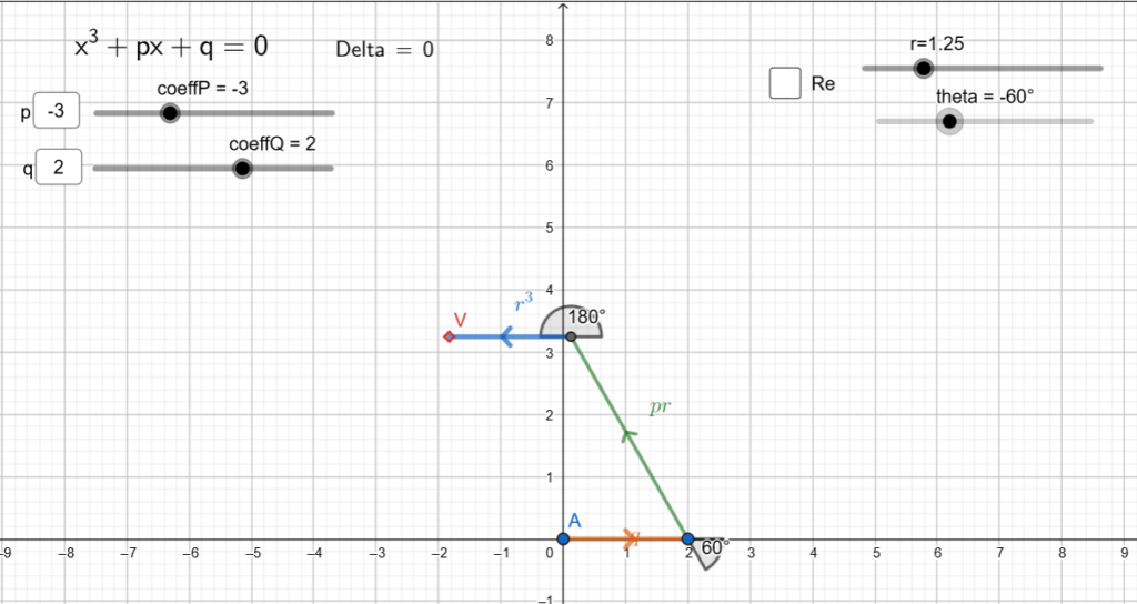
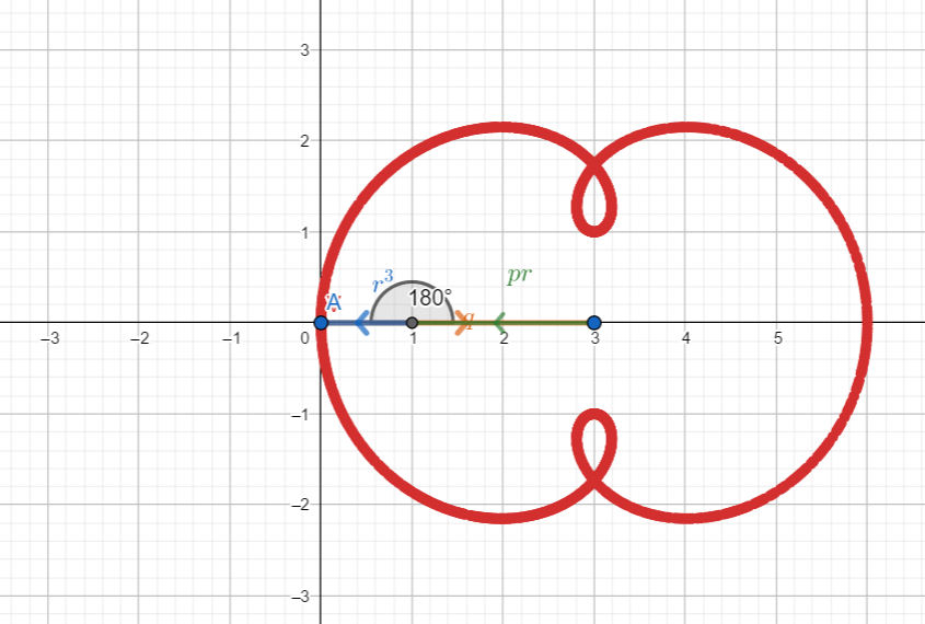
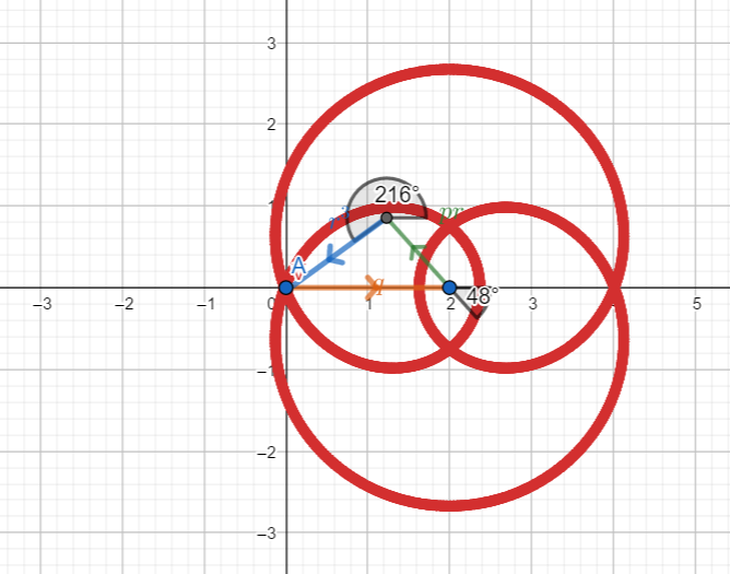
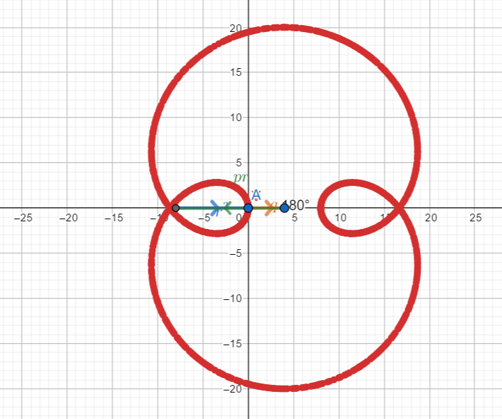
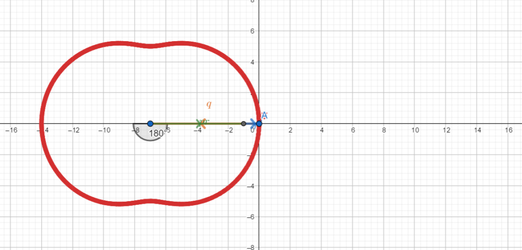
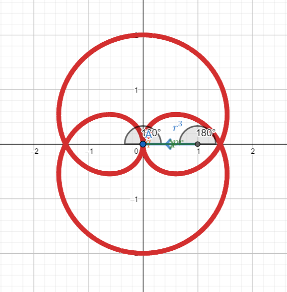
Whatever the combination of the coefficients, we note that while the angle $\theta$ sweeps the whole range from $-180^\circ$ to $180^\circ$ , the green segment (which corresponds to the linear term) , makes a turn while the blue one (which corresponds to the cubic term) makes three turns. The situation is somewhat reminiscent of the Ptolemaic system, with its deferents and epicycles, and in fact the curve described by the vertex, with $\rho$ fixed, is a two-lobed epitrochoid.

First of all it is convenient to search for the real solutions, then put the angle slider $\theta$ on the values $0^\circ$ (positive real solutions) and then $-180^\circ$ or $180^\circ$ for the any real negative solutions. Once the real solution or solutions have been identified, the remaining ones can be searched for, in accordance with the following table:

	$\Delta < 0$	$\Delta = 0$	$\Delta > 0$
real solutions	three, distinct	three, at least two coincidents	one only

There is a method that simplifies the search for pairs of complex solutions: just solve this triangle:

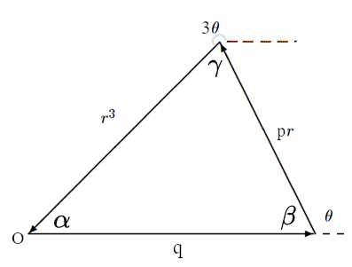
We will find that the following relations hold:
$\beta = \pi - \theta$
$\gamma = 2 \pi - (\pi - \theta) - 3 \theta = \pi - 2 \theta$
$\alpha = \pi - (\pi - \theta) - (\pi - 2 \theta) = 3 \theta - \pi$

therefore the relation that characterizes the triangle solution of the reduced equation of the third degree is:
$2 \beta - \gamma = \pi$
or also
$\theta = \pi / 2 - \gamma /2$
and it will be enough to apply the sine theorem to find $r$ as a function of $\theta$ :

$\begin{equation} \frac{pr}{\sin \alpha} = \frac{q}{\sin \gamma}$

$\begin{equation} \frac{pr}{\sin (3 \theta - \pi)} = \frac{q}{\sin (\pi - 2 \theta)}$

$\begin{equation} r = \frac{q \sin (3 \theta - \pi)}{p \sin (\pi - 2 \theta)}$

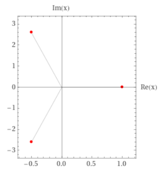
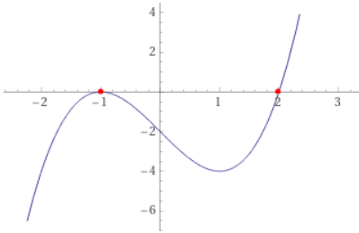
Example 1 – positive delta: one real solution only

$x^3 + 2x + 3 = 0$
$\Delta = 2.6$
$x_1 = -1$
$x_{2,3} = (1 \pm i \sqrt 11) / 2$

The two complex conjugate solutions originate from two different lobes of the curve

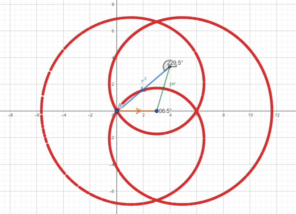
Example 2 – similar to the previous case

$x^3 - x + 2 = 0$
$\Delta = 0.96$
$x_1 = -1.52$
$x_{2,3} = 0.761 \pm i 0.858$

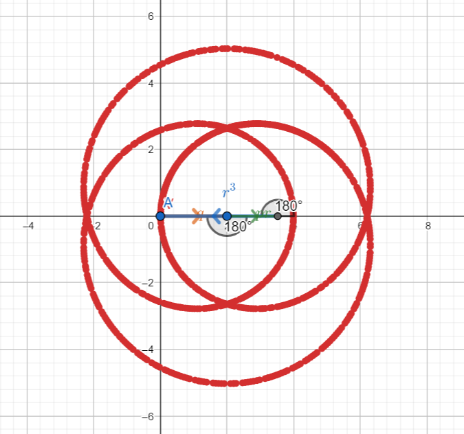
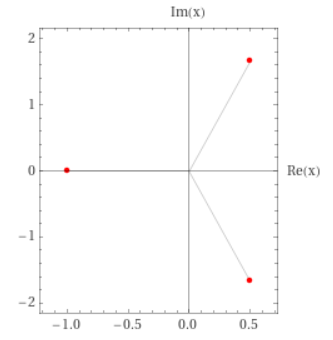
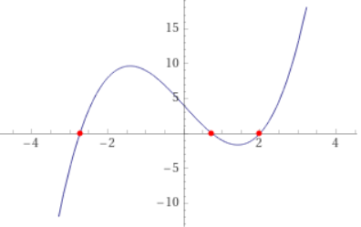
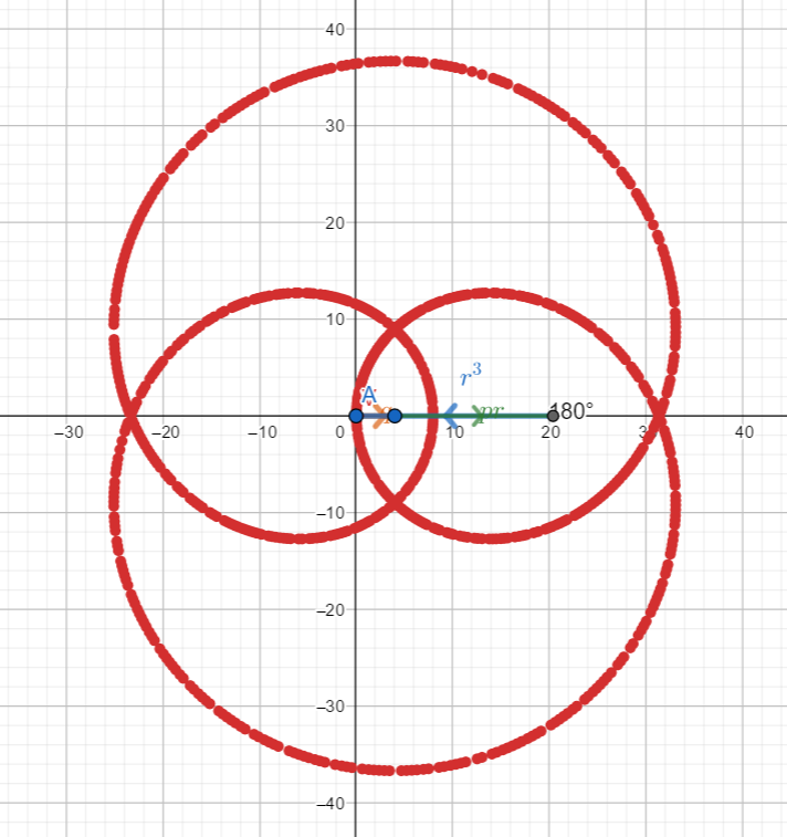
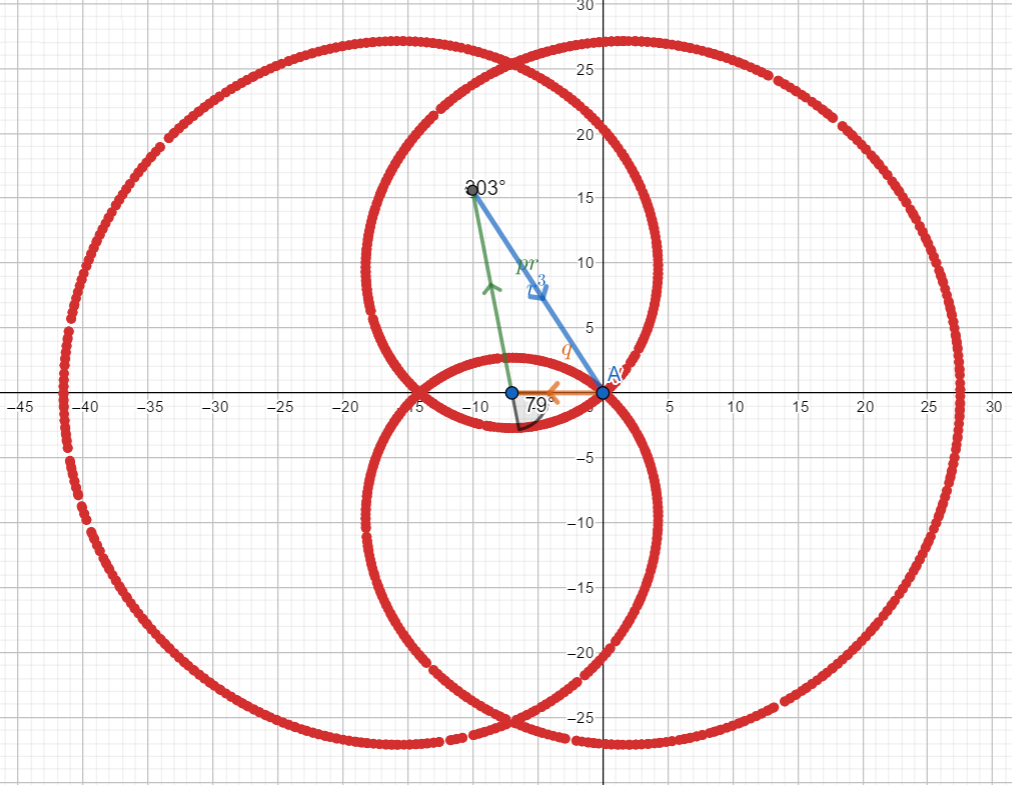
Example 3 – negative delta: three real solutions

$x^3 - x = 0$
$\Delta = -1/27$
$x_1 = 0; x_2 = -1; x_3 = +1$

The two solutions with $\rho = 1$ derive from two distinct branches of the curve and the degenerate solution $x = 0$

Example 4 – similar to the previous case but three distinct curves

$x^3 - 6x + 4 = 0$
$\Delta = -4.2$
$x_1 = 2$
$x_{2,3} = -1 \pm \sqrt 3$

Example 5 – similar to (1) and (2)

$x^3 + 6x - 7 = 0$
$\Delta = 81/4$
$x_1 = 1$
$x_{2,3} = (-1 \pm 3i \sqrt 3) / 2$

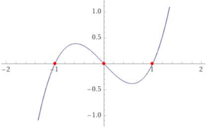
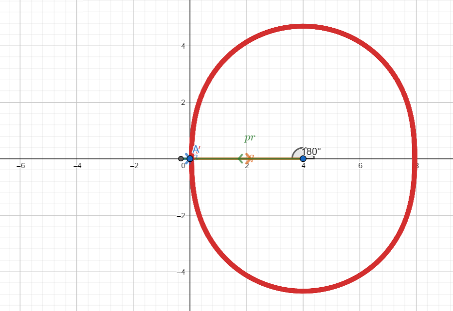
Example 6 – null delta: three real solutions having at least two coincident

$x^3 - 3x - 2 = 0$
$\Delta = 0$
$x_1 = x_2 = -1$
$x_3 = 2$

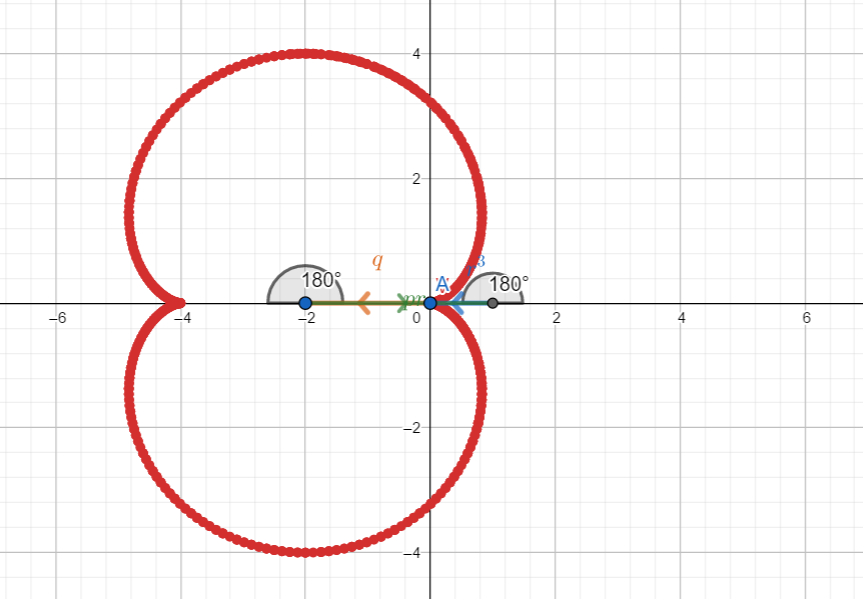The two coincident solutions with $\rho = -1$ : the curve doesn’t have a loop but a stationary point on real axis, thus the solution has double multiplicity. **[is it an epicycloid in that case (?)]**

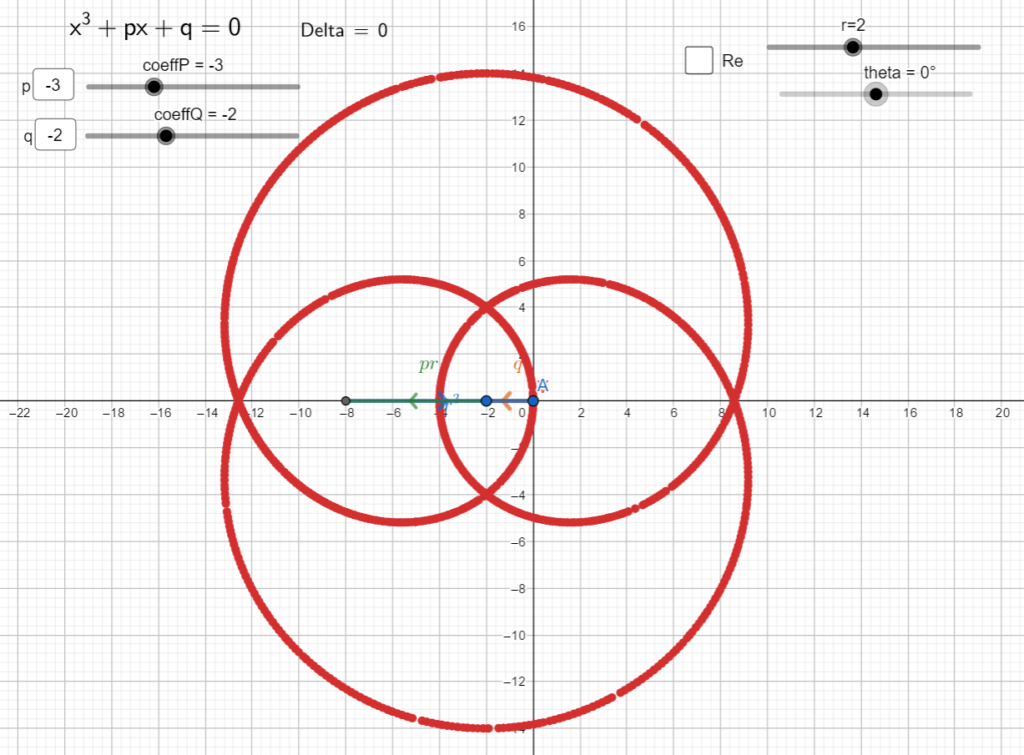
The only equation with three coincident real solutions is in the form $(x-k)^3 = 0$ , which in the reduced form transformation becomes $x^3 = 0$ whose solution is a point in the origin with multiplicity 3.